home   Java Script   MS Access   Perl   HTML   Delphi   C ++   Visual Basic   Java   CGIPerl   MS Excel   Front Page 98   Windows 98   Ms Word   Builder   PHP   Assembler     Link to us   Links    


Using Numbers, Formulas, and Functions with Excel 97

What you will learn from this lesson

With Excel 97 you will:


What you should do before you start this lesson

  1. Start Excel 97.
  2. Open a new worksheet.


Exploring the lesson

You can create worksheets to record and calculate grades using Excel 97. The power of Excel 97 is great. Not only can Excel 97 calculate student grades, weighted scores, and program-planning budgets, but it also can maintain the financial records of an entire school. For this lesson, you will explore some basic functions that you can use in your classroom.

Sorting functions of Excel 97

Recording names and addresses of your students can be a full-time job. Just as soon as you have everyone in the correct order, you have a new student whose last name starts with the letter C. With Excel 97, sorting the names by last name, by the enrollment date, or even by birthday is quick and easy.

There are many details to track in a classroom, such as student data, grades, project progress, student participation, homework, and other completed assignments. Using Excel 97, you can track all this information for each student, and then organize it according to importance or category.

Alphabetizing names

  1. Starting with the column headings in cell A3, create a list of student names on your worksheet. Enter each name, e-mail address, and classroom seating assignment in separate columns, similar to the example shown below. Use the tab key to move across each row cell by cell, and the enter or down-arrow key to move down in each column.
  2. #

    A

    B

    C

    3

    Name

    e-mail address

    Seating

    4

    Juanita

    juanita@washington.k12.wa.us

    R2-3

    5

    John

    john@ washington.k12.wa.us

    R2-1

    6

    Roy

    roy@ washington.k12.wa.us

    R1-1

    7

    Tom

    tom@ washington.k12.wa.us

    R1-3

    8

    Kim

    kim@ washington.k12.wa.us

    R1-2

    9

    Sean

    sean@ washington.k12.wa.us

    R3-1

    10

    Georgia

    georgia@ washington.k12.wa.us

    R2-1

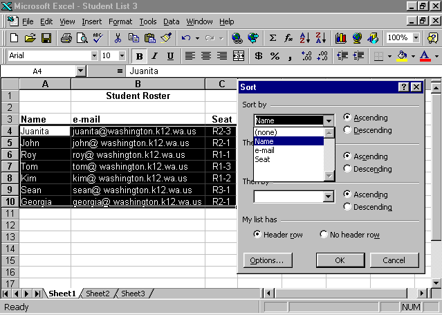
  3. Select the data table.
  4. On the Data menu, click Sort.
  5. Under Sort by, select Name, and then click Ascending.
  6. Click OK.
  7. Save your file with the name Student List for use later to record test scores.
  8. Close the workbook.


Creating a one-input data table

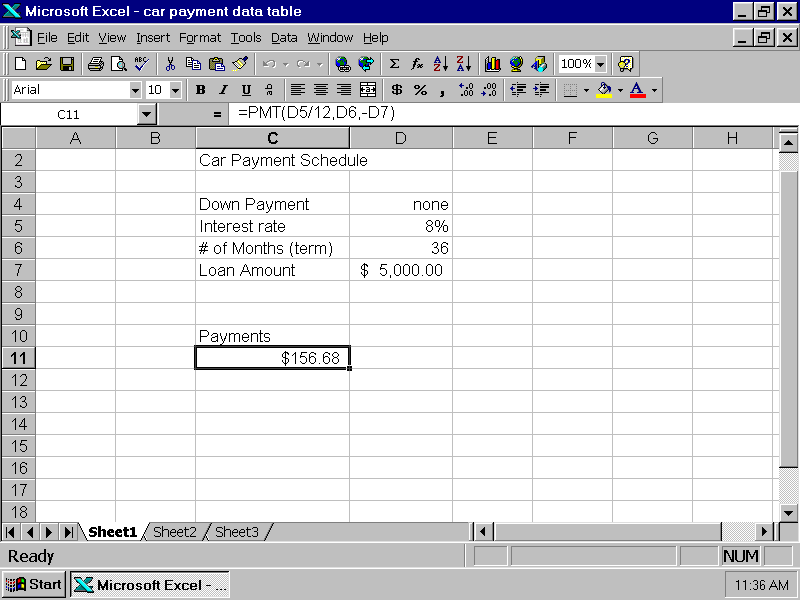
Using Excel 97, you and your students can learn the costs associated with making payments on purchases. You can easily calculate monthly payments based on interest and balance due on purchases. In the next exercise, you can calculate monthly payments based on interest and total cost of a car, showing how the loan term and interest rates affect monthly payments.

Calculating car payments

  1. Open a new workbook.
  2. Click Sheet2 at the bottom of the window.
  3. In cell C2, type Car Payment Schedule.
  4. Type the following text and formulas in the cells shown in the chart:
  5. Row #

    Column C

    Column D

    2

    Car Payment Schedule


    3


    4

    Down Payment

    None

    5

    Interest Rate

    8%

    6

    # of Months (term)

    36

    7

    Loan Amount

    $5000

    8


    9


    10

    Payments


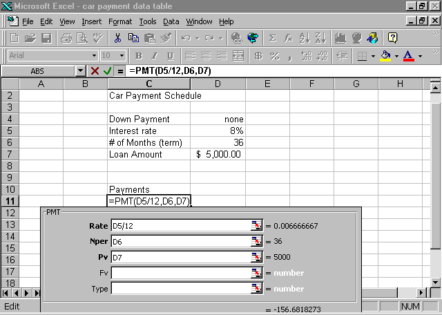
  6. Click cell C11, and on the Formula toolbar, click the Edit Formula button (the = sign).
  7. Click the Functions arrow, and click PMT, if visible.
    – or –
    Click More Functions.
  8. In the Function category, click Financial.
  9. In the Function name, click PMT, and then click OK.
  10. Click the Shrink button at the right of the input area, click D5 on the worksheet, and then press enter.
  11. In the Rate box, click after D5, and type /12.
  12. Click the Nper window, and click the Shrink button.
  13. Click D6 on the worksheet, and press enter.
  14. Click the Pv window, and click the Shrink button.
  15. Click D7 on the worksheet, and press enter.
  16. Click OK.
  17. To change the months of the loan to 24, type 24 in cell D5.
  18. To change the interest rate to 12.5 percent to demonstrate how the payment changes, type 12.5 in cell D4. Try several combinations on your own, and see how it works.
  19. Close the workbook without saving it.

Order of calculation in Excel 97

You have just discovered one easy formula in Excel 97. There are many others that help you calculate or analyze everything from finances to statistical sampling plans. When you combine several mathematical steps in a formula, they are performed in a specific order. Excel 97 will start calculating from the left to the right according to the following order of operations:

For reference, the Comparison operators are:


Hiding columns

Using Excel 97 to maintain all of your student records in one file is handy but sometimes awkward. Hiding columns is an easy technique to “fold” away columns you may need, but not need to see for a particular process such as recording test scores and grades. You will find this technique very useful in maintaining complete records in one file.

Hiding columns with test scores
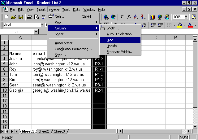
  1. Open the Student List workbook.
  2. Click the column C header to select the column.
  3. On the Format menu, position the pointer on Column, and click Hide.
  4. To unhide your columns, on the Format menu, position the pointer on Column, and click Unhide.
  5. Close the workbook without saving.


Calculating grades for equal tests

When all tests are equal, you can easily add the raw data, calculate the average, and determine the grade. Assume that you are grading on a specific range of points for each letter grade. The scale is 90–100=A, 80–89=B, 70–79=C, and 60–69=D. Any score less than 60 is an F.

Average function

In this exercise you have given your students equal weekly tests over two months and want to calculate their average grades.

Averaging test scores

  1. Open the Student List workbook, and enter the following dates and raw test scores. Start by typing 9/1 in cell D3.
  2. Name

    9/1

    9/8

    9/15

    9/22

    9/29

    10/6

    10/13

    10/20

    Juanita

    93

    97

    89

    94

    88

    92

    93

    95

    John

    95

    85

    83

    93

    87

    85

    91

    90

    Roy

    97

    95

    92

    96

    91

    93

    98

    99

    Tom

    85

    80

    87

    83

    88

    84

    82

    90

    Kim

    87

    84

    90

    88

    86

    82

    91

    92

    Sean

    88

    95

    94

    95

    91

    85

    90

    93

    Georgia

    91

    86

    89

    89

    90

    94

    88

    96

  3. Hide column B and column C.
  4. In cell L3, type Quiz Ave.
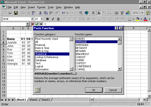
  5. Move the pointer to cell L4, and on the Standard toolbar click Paste Function.
  6. Under the Function category, click Statistical; under Function name, select Average, and click OK.
  7. Click OK to complete the function and average one row of grades.
  8. Click Save--

Copying formulas

Once you have created a formula, you can quickly and easily copy it into adjacent cells to calculate student records that contain the same type of data.

Copying formulas
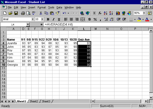
  1. Using the worksheet from the previous lesson, click the L4 cell to select it.
  2. Click and drag the fill handle at the lower-right corner of the cell to the bottom of the column, and release the pointer.
  3. Save your file with the name Student List.

Applying a formula to equally weighted tests

Now that you have recorded test scores and calculated averages, you can easily figure letter grades from numbered scores using Excel 97.

For this type of formula, Excel 97 compares data with a formula that evaluates the data to a logical value of true (1) or false (0). Using Excel 97 to calculate grades is quick and easy. The formula interprets a range of data such as >89 (which means 90 or more) and assigns a letter grade if the data meets the criteria (score is >89—true or false). Therefore, you have a conditional calculation commonly known as an If-Then statement for equally weighted tests.

Creating letter grades from number scores
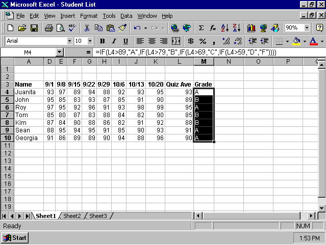
  1. Open the file named Student List that was saved from the previous exercise.
  2. Position the pointer in cell M3, type Grade, and then reclick M3.
  3. On the Formatting toolbar, click the Bold button to make the heading bold.
  4. Click cell M4, and enter the following, very carefully: =IF(L3>89,"A",IF(L3>79,"B",IF(L3>69,"C",IF(L3>59,"D","F"))))
  5. Click and drag the fill handle in cell M4 to cell M10.
  6. Save the workbook.


Analyzing scores

Sometimes the tests and assignments you give are not equal in importance, making the grading process more complex. Excel 97 can help you analyze these types of test scores.

Calculating mean, median, and standard deviation for each test
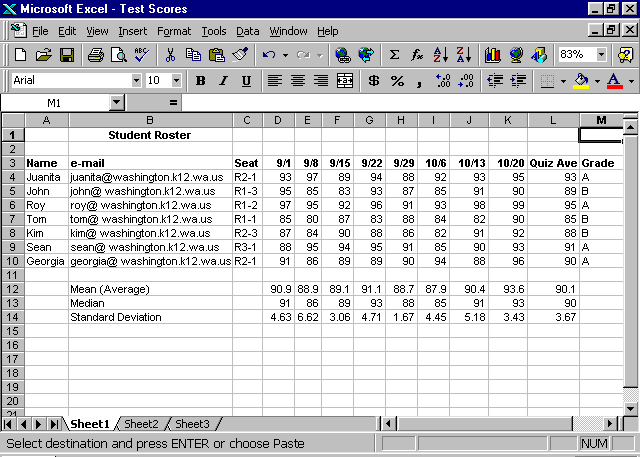
  1. Continuing in your Student ist workbook, click cell B12, and type Average.
  2. Click cell B13, and type Median.
  3. Click cell B14, and type Standard Deviation.
  4. Click cell D12, and on the Standard toolbar click Paste Function.
  5. In the Function category, make sure Statistics is selected, and in the Function type, click Average, and then click OK.
  6. If D4:D10 is not in Number1, type it in.
  7. Click OK.
  8. Click cell D13.
  9. On the Insert menu, click Function.
  10. In the Function category, click Statistics, and in the Function type, click Median, and then click OK.
  11. If D4:D10 is not in Number1, type it in.
  12. Click OK.
  13. Click cell D14, and type =STDEVP(D4:D10).
  14. Select cells D12, D13, and D14.
  15. Click and drag the fill handle to column L.
  16. Right-click the row header 12, and click Format Cells.
  17. In Decimal places, type 1.
  18. Adjust the decimal to 2 places for the Standard Deviation.
  19. In Decimal places, type 2.
  20. Save the workbook.


Creating a budget for a school function

Having a successful school function often depends on having a budget in place. For this exercise you will create a budget and test to see what happens to the results when you change any of the components.

Entering budget categories

Creating a budget involves entering the categories and specific items into the worksheet. The first step to creating a budget in Excel 97 is to determine the budget categories and enter them in the worksheet.

Entering categories for a budget

  1. Open a new workbook, and save it with the name Budget.
  2. Click cell A2, type the title Budget: Awards Dinner, click Budget, and then, on the Formatting toolbar, click the Bold button.
  3. Increase the width of column A to 23.
  4. Click Budget, drag it to cell D2, and then click the Merge and Center button.
  5. Click cell B3, and type Items; click cell C3, and type Budget; and in cell D3, type Actual.
  6. Click cell A4, and type Supplies; click cell B4, and type Paper Products; and then click cell B5, and type Decorations.
  7. Double-click between columns B and C to fit the text to the cell.
  8. Click cell A7, and type Food; click cell B7, and type Meals; and click cell B8, and type Beverages.
  9. Click cell A10, and type Awards; click cell B10, and type Certificates.
  10. Click cell A13, and type Miscellaneous; and then click cell B13, and type Custodial.
  11. Click in cell A16, and type Totals; on the Formatting toolbar, click the Align Right button.
  12. Click cell B3, drag it to cell D3, and then click the Bold button on the Formatting toolbar.
  13. Click cell A4, drag it to cell A16, and then click the Bold button on the Formatting toolbar.

Entering budgeted amounts and formulas

The next step in preparing a budget for the Awards Dinner is to determine budget amounts and place them with formulas in the worksheet.

Placing budgeted amounts in formulas

  1. In the Budget workbook from the previous lesson, click cell C4 and type 50.00.
  2. Click cell C5, and type 25.00.
  3. Click cell C7, and type 250.00.
  4. Click cell C8, and type 30.00.
  5. Click cell C10, and type 75.00.
  6. Click cell C13, and type 65.00.
  7. Click cell C4, drag it to cell C16, and then click Currency Style ($).
  8. Click cell C16, click the Edit Formula button (the = sign), and on the Formula bar, click Sum.
  9. In Sum Number1, type C4:C13, and click OK.

Entering actual amounts

The final step in using Excel 97 to budget the Awards Dinner is to record the actual amounts spent. Using Excel 97 to budget an event helps track current expenses and makes it easy to plan future events using the same budget process. As you receive and pay the invoices for your Awards Dinner, enter the values into your budget worksheet.

Completing the budget process with actual amounts
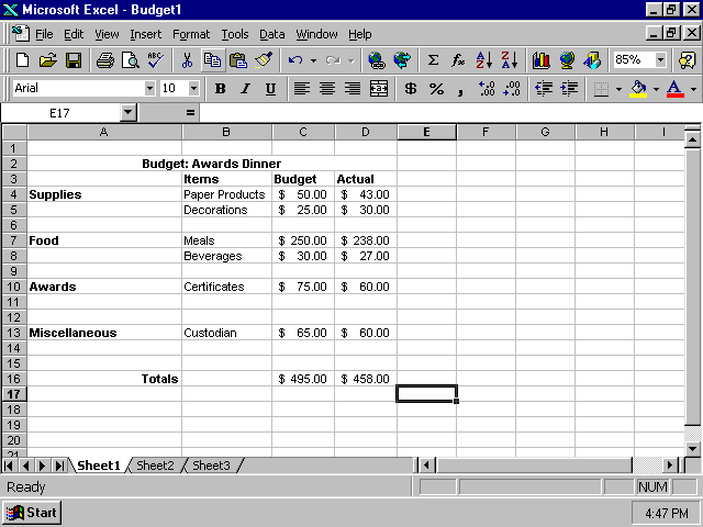
  1. In the Budget workbook from the previous lesson, click cell D4, and type 43.00.
  2. Click cell D5, and type 30.00.
  3. Click cell D7, and type 238.00.
  4. Click cell D8, and type 27.00.
  5. Click cell D10, and type 60.00.
  6. Click cell D13, and type 60.00.
  1. Click cell D4, drag it to cell D16, and then click the Currency Style button ($).
  2. Click cell C16, drag it to cell D17, and then press enter.
  3. Save the workbook.


How you can use what you learned

As you become more comfortable with worksheets, you will discover many applications for them. Using Excel 97 you can easily and quickly maintain student records. Students can reinforce basic mathematical processes using Excel 97 to produce charts and tables. Furthermore, by adding well-designed charts and tables to reports, students can enhance both their understanding of the content and their presentation of the information. In addition, you can also check student math problems.


Extensions

Exploring the Roman numeral function

Converting Roman numerals is an exercise in logic. Explain to your students that if we were still using Roman numerals, the year 2000 would be easy to represent with the letters MM.

Converting years from Arabic to Roman numerals
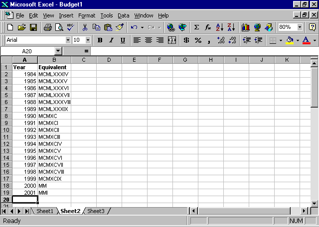
  1. Open a new workbook.
  2. In cell A1, type Year.
  3. Tab to cell B1, type Equivalent, and then click enter.
  4. Make cells A1 and B1 bold, and then double-click between columns B and C.
  5. Click cell A2, type 1984, and then press enter.
  6. In cell A3, type 1985, and then press enter.
  7. Select cells A2 and A3, and drag the fill handle to cell A19.
  8. Click cell B2.
  9. On the Standard toolbar, click the Paste Function button.
  10. Click Math & Trig, and in the Function name, click Roman.
  11. Click cell A2.
    – or –
    Type A2 in the Number window.
  12. Type 0 in the Form window (for Classical Roman numerals), and then click OK.
  13. Select cell B2, and drag the fill handle to cell B19.
  14. Close the workbook without saving changes.


Summarizing what you learned

In this chapter you explored and practiced:

scores.